You have 2 free member-only stories left this month.

Sign up for Medium and get an extra one

All Pandas cut() you should know for transforming numerical data into categorical data

B. Chen

Feb 8·6 min read

All Pandas cut() you should know for transforming numerical data into categorical data (Image by author using canva.com)

Numerical data is common in data analysis. Often you have numerical data that is continuous, very large scales, or highly skewed. Sometimes, it can be easier to bin those data into discrete intervals. This is helpful to perform descriptive statistics when values are divided into meaningful categories. For example, we can divide the exact age into Toddler, Child, Adult, and Elder.

Pandas’ built-in cut() function is a great way to transform numerical data into categorical data. In this article, you’ll learn how to use it to deal with the following common tasks.

1. Discretizing into equal-sized bins
2. Adding custom bins
3. Adding labels to bins
4. Configuring leftmost edge with right=False
5. Include the lowest value with include_lowest=True
6. Passing an IntervalIndex to bins
7. Returning bins with retbins=True
8. Creating unordered categories

Please check out Notebook for the source code.

1. Discretizing into equal-sized bins

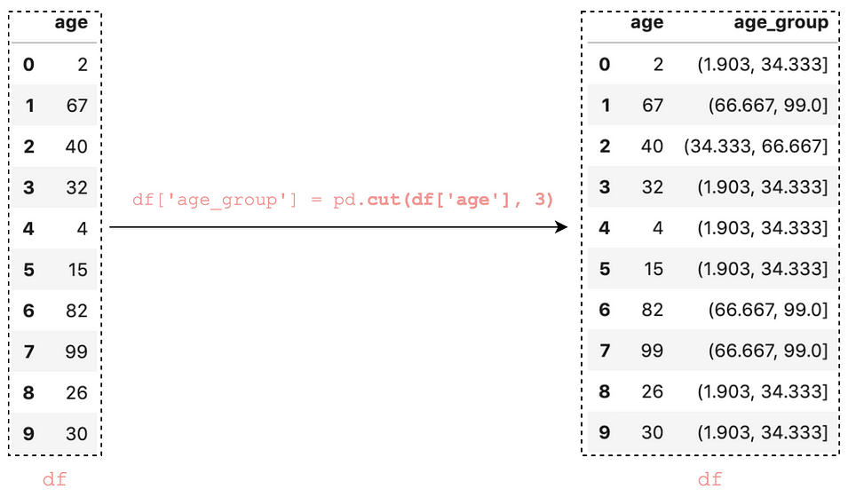
The simplest usage of cut() must has a column and an integer as input. It is discretizing values into equal-sized bins.

df = pd.DataFrame({'age': [2, 67, 40, 32, 4, 15, 82, 99, 26, 30]})df['age_group'] = pd.cut(df['age'], 3)

(image by author)

Did you observe those intervals from the age_group column? Those interval values are having a round bracket at the start and a square bracket at the end, for example (1.903, 34.333]. It basically means any value on the side of the round bracket is not included in the interval and any value on the side of the square bracket is included (It is known as open and closed intervals in Math).

Now, let's take a look at the new column age_group.

df['age_group']

(image by author)

It shows dtype: category with 3 label values: (1.903, 34.333] , (34.333, 66.667] , and (66.667, 99.0]. Those label values are ordered as indicated with the symbol <. Behind the theme, an interval is calculated as follows in order to generate the equal-sized bins:

interval = (max_value — min_value) / num_of_bins
         = (99 - 2) / 3
         = 32.33333        (<--32.3333-->] < (<--32.3333-->] < (<--32.3333-->]        (1.903, 34.333] < (34.333, 66.667] < (66.667, 99.0]

2. Adding custom bins

Let’s divide the above age values into 4 custom groups i.e. 0–12, 12–19, 19–60, 61–100. To do that, we can simply pass those values in a list ([0, 12, 19, 61, 100]) to the argument bins.

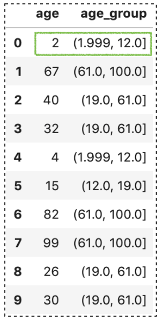
df['age_group'] = pd.cut(df['age'], bins=[0, 12, 19, 61, 100])

(image by author)

We added the group values for age in a new column age_group. By looking into the column

df['age_group']0      (0, 12]
1    (61, 100]
2     (19, 61]
3     (19, 61]
4      (0, 12]
5     (12, 19]
6    (61, 100]
7    (61, 100]
8     (19, 61]
9     (19, 61]
Name: age_group, dtype: category
Categories (4, interval[int64]): [(0, 12] < (12, 19] < (19, 61] < (61, 100]]

We can see dtype: category with 4 ordered label values: (0, 12] < (12, 19] < (19, 61] < (61, 100].

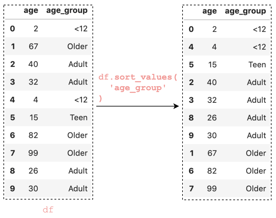
Let’s sort the DataFrame by the column age_group:

df.sort_values('age_group')

(image by author)

Let’s count that how many values fall into each bin.

df['age_group'].value_counts().sort_index()(0, 12]      2
(12, 19]     1
(19, 61]     4
(61, 100]    3
Name: age_group, dtype: int64

3. Adding labels to bins

It is more descriptive to label these age_group values as ‘<12’, ‘Teen’, ‘Adult’, ‘Older’. To do that, we can simply pass those values in a list to the argument labels

bins=[0, 12, 19, 61, 100]
labels=['<12', 'Teen', 'Adult', 'Older']df['age_group'] = pd.cut(df['age'], bins, labels=labels)

(image by author)

Now, when we looking into the column, it shows the label instead

df['age_group']0      <12
1    Older
2    Adult
3    Adult
4      <12
5     Teen
6    Older
7    Older
8    Adult
9    Adult
Name: age_group, dtype: category
Categories (4, object): ['<12' < 'Teen' < 'Adult' < 'Older']

Similarly, it is showing label when sorting and counting

(image by author)

df['age_group'].value_counts().sort_index()<12      2
Teen     1
Adult    4
Older    3
Name: age_group, dtype: int64

4. Configuring leftmost edge with right=False

There is an argument right in Pandas cut() to configure whether bins include the rightmost edge or not. right defaults to True, which mean bins like[0, 12, 19, 61, 100] indicate (0,12], (12,19], (19,61],(61,100] . To include the leftmost edge, we can set right=False:

pd.cut(df['age'], bins=[0, 12, 19, 61, 100], right=False)0      [0, 12)
1    [61, 100)
2     [19, 61)
3     [19, 61)
4      [0, 12)
5     [12, 19)
6    [61, 100)
7    [61, 100)
8     [19, 61)
9     [19, 61)
Name: age, dtype: category
Categories (4, interval[int64]): [[0, 12) < [12, 19) < [19, 61) < [61, 100)]

5. Including the lowest value with include_lowest=True

Suppose you would like to divide the above age values into 2–12, 12–19, 19–60, 61–100 instead. You will get a result contains NaN when setting the bins to [2, 12, 19, 61, 100].

df['age_group'] = pd.cut(df['age'], bins=[2, 12, 19, 61, 100])

(image by author)

We get a NaN because the value 2 is the leftmost edge of the first bin (2.0, 19.0] and is not included. To include the lowest value, we can set include_lowest=True. Alternatively, you can set the right to False to include the leftmost edge.

df['age_group'] = pd.cut(
    df['age'], 
    bins=[2, 12, 19, 61, 100], 
    include_lowest=True
)

(image by author)

6. Passing an IntervalIndex to bins

So far we have been passing an array to bins. Instead of an array, we can also pass an IntervalIndex.

Let’s create an IntervalIndex with 3 bins (0, 12], (19, 61], (61, 100] :

bins = pd.IntervalIndex.from_tuples([(0, 12), (19, 61), (61, 100)])
IntervalIndex([(0, 12], (19, 61], (61, 100]],
              closed='right',
              dtype='interval[int64]')

Next, let’s pass it to the argument bins

df['age_group'] = pd.cut(df['age'], bins)

(image by author)

Notice that value not covered by the IntervalIndex is set to NaN. Basically, passing an IntervalIndex for bins results in those categories exactly.

7. Returning bins with retbins=True

There is an argument called retbin to return the bins. If it is set to True, the result will return the bins and it is useful when bins is passed as a single number value

result, bins = pd.cut(
    df['age'], 
    bins=4,            # A single number value
    retbins=True
)
# Print out bins value
bins
array([ 1.903, 26.25 , 50.5  , 74.75 , 99.   ])

8. Creating unordered categories

ordered=False will result in unordered categories when labels are passed. This parameter can be used to allow non-unique labels:

pd.cut(
    df['age'], 
    bins=[0, 12, 19, 61, 100], 
    labels=['<12', 'Teen', 'Adult', 'Older'], 
    ordered=False,
)0      <12
1    Older
2    Adult
3    Adult
4      <12
5     Teen
6    Older
7    Older
8    Adult
9    Adult
Name: age, dtype: category
Categories (4, object): ['<12', 'Teen', 'Adult', 'Older']

Conclusion

Pandas cut() function is a quick and convenient way for transforming numerical data into categorical data.

I hope this article will help you to save time in learning Pandas. I recommend you to check out the documentation for the cut() API and to know about other things you can do.

Thanks for reading. Please check out the notebook for the source code and stay tuned if you are interested in the practical aspect of machine learning.

You may be interested in some of my other Pandas articles:

• A Practical Introduction to Pandas Series
• Using Pandas method chaining to improve code readability
• How to do a Custom Sort on Pandas DataFrame
• All the Pandas shift() you should know for data analysis
• When to use Pandas transform() function
• Pandas concat() tricks you should know
• Difference between apply() and transform() in Pandas
• All the Pandas merge() you should know
• Working with datetime in Pandas DataFrame
• Pandas read_csv() tricks you should know
• 4 tricks you should know to parse date columns with Pandas read_csv()

More tutorials can be found on my Github

Quantity : Add to Cart